How To Freeze Cells In Excel: While working with bigger spreadsheets, you should know how to freeze cells in Excel. You don’t have to look all over more than once, rather simply freeze the cells to contrast the header data and whatever is left of the columns rapidly. Along these lines, here, we disclose to you the technique to freeze cells in Excel.
Note: In this guide, we have used Microsoft Office Professional Plus 2016 version. The steps to freeze the cells would continue as before dated back to Excel’s 2010 version.
How To Freeze Cells In Excel?
1. The Top Row – Freeze Cells In Excel
If you are certain that you need to freeze the highest line in the spreadsheet, this is what you have to do:
Step By Steps Instruction To Freeze Top Row In Excel
- Open the coveted spreadsheet in Excel.
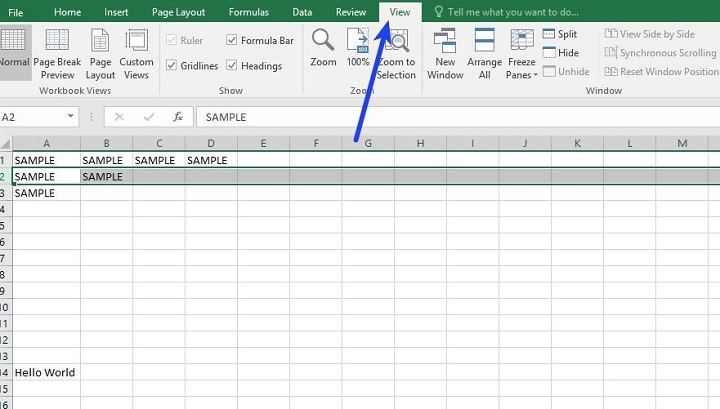
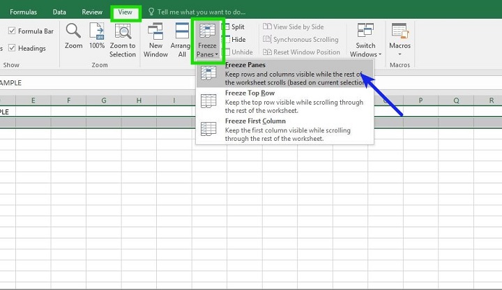
2. Simply, explore the “View” tab on the menu bar.
3. Now, you will watch an option that says – “Freeze Panes” on it. Just, tap on it to see more options.
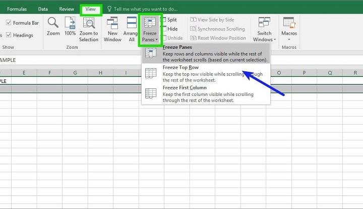
4. Finally, from the options, you have to choose “Freeze Top Row” with a specific end goal to solidify the highest line of your excel sheet.
How to Authorize A Computer on iTunes
2. The First Column – Freeze Cells In Excel
Like the past method, in the event that you have to freeze the 1st column of the excel sheet, you have to take after the steps mentioned beneath.
Step By Steps Instruction To Freeze The First Column In Excel
1.Open the coveted spreadsheet in Excel.
2. Simply, explore the “View” tab on the menu bar.

3. Then, you will watch an option that says – “Freeze Panes” on it. Just, tap on it to see more options.
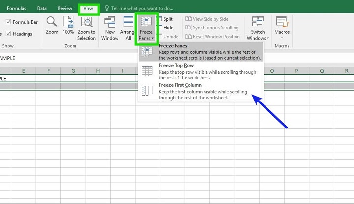
4. Finally, from the options, you have to choose “Freeze First Column” with a specific end goal to freeze the 1st column of your excel sheet.
How To Delete Instagram Account
3. Desired Row – Freeze Cells in Excel
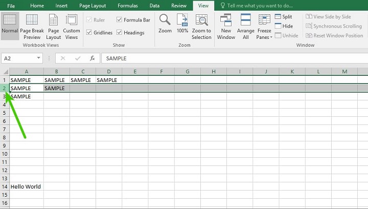
Before freezing the cells, for this situation, you have to first choose the whole column. Here are the steps for how you can freeze a total row:
Step by Steps Instruction To Freeze The Selected Row In Excel
1. Open the coveted spreadsheet in Excel.
2. First of all, you have to choose the row you have to freeze. So as to choose the whole line, you have to tap on the column number (said to one side of each line).
3. Simply, explore the “View” tab on the menu bar.

4. Then, you will watch an option that says – “Freeze Panes” on it. Just, tap on it to see more options.
5. Finally, from the options, you have to choose “Freeze Panes” with a specific end goal to solidify the line you chose already.
How to Extract RAR files (Windows+Mac)
4. Desired Column – Freeze Cells In Excel
For this situation, each of the steps said above will precisely be the same. But, you have to choose a whole column to freeze instead of a row.